Difference between revisions of "Theory Notes"
m |
(→The Hartree Fock Method) |
||
| Line 44: | Line 44: | ||
For purposes of comparison, and to define the correlation energy, assume that <math>\psi({\bf r}_1,{\bf r}_2)</math> can be written in the separable product form | For purposes of comparison, and to define the correlation energy, assume that <math>\psi({\bf r}_1,{\bf r}_2)</math> can be written in the separable product form | ||
\begin{equation} | \begin{equation} | ||
| − | \psi({\bf r}_1,{\bf r}_2) = \frac{1}{\sqrt{2}}[u_1(r_1)u_2(r_2) \pm u_2(r_1)u_1(r_2)]\nonumber | + | \psi({\bf r}_1,{\bf r}_2) = \frac{1}{\sqrt{2}} \left[ u_1(r_1) u_2(r_2) \pm u_2(r_1) u_1(r_2) \right] \nonumber |
\end{equation} | \end{equation} | ||
| − | for the <math>1s^2\ ^1\!S</math> ground state. Because of the | + | for the <math>1s^2\ ^1\!S</math> ground state. Because of the $\frac{1}{r_{12}}$ term in the Schrödinger equation, the exact solution connot be expressed in this form as a separable product. However, the Hartree-Fock approximation corresponds to finding the best possible solution to the Schrödinger equation |
\begin{equation} | \begin{equation} | ||
| − | H\psi( | + | H\psi({\bf r}_1,{\bf r}_2) = E\psi({\bf r}_1,{\bf r}_2)\nonumber |
\end{equation} | \end{equation} | ||
that can nevertheless be expressed in this separable product form, where as before | that can nevertheless be expressed in this separable product form, where as before | ||
| Line 54: | Line 54: | ||
H = -\frac{1}{2}(\nabla^2_1+\nabla^2_2) - \frac{1}{r_1}- \frac{1}{r_2} + \frac{Z^{-1}}{r_{12}}\nonumber | H = -\frac{1}{2}(\nabla^2_1+\nabla^2_2) - \frac{1}{r_1}- \frac{1}{r_2} + \frac{Z^{-1}}{r_{12}}\nonumber | ||
\end{equation} | \end{equation} | ||
| − | is the full two-electron Hamiltonian. To find the best solution, substitute into <math>\langle\psi | + | is the full two-electron Hamiltonian. To find the best solution, substitute into <math>\left\langle\psi \lvert H-E \rvert \psi\right\rangle</math> and require this expression to be stationary |
with respect to arbitrary infinitesimal variations <math>\delta u_1</math> and <math>\delta | with respect to arbitrary infinitesimal variations <math>\delta u_1</math> and <math>\delta | ||
| − | u_2</math> in <math>u_1</math> and <math>u_2</math>; i.e. | + | u_2</math> in <math>u_1</math> and <math>u_2</math> respectively; i.e. |
\begin{equation} | \begin{equation} | ||
| − | \frac{1}{2}\langle\delta u_1(r_1)u_2(r_2) \pm u_2(r_1)\delta | + | \frac{1}{2} \left\langle \delta u_1(r_1)u_2(r_2) \pm u_2(r_1)\delta |
| − | u_1(r_2) | + | u_1(r_2) \lvert H-E \rvert u_1(r_1) u_2(r_2)\pm u_2(r_1) u_1(r_2)\right\rangle\nonumber |
\end{equation} | \end{equation} | ||
\begin{equation} | \begin{equation} | ||
| − | =\int\delta u_1(r_1)d{\bf r}_1\{\int d{\bf r} | + | =\int\delta u_1(r_1) d{\bf r}_1 \left\{ \int d{\bf r}_2 u_2(r_2) \left( H - E \right) \left[ u_1(r_1)u_2(r_2) \pm u_2(r_1) u_1(r_2) \right] \right\}\nonumber |
\end{equation} | \end{equation} | ||
| Line 76: | Line 76: | ||
\begin{equation} | \begin{equation} | ||
| − | \int d{\bf r}_1 u_1(r_1)(H-E)[u_1(r_1)u_2(r_2) \pm | + | \int d{\bf r}_1 u_1(r_1) \left( H-E \right) \left[ u_1(r_1) u_2(r_2) \pm |
| − | u_2(r_1)u_1(r_2)] = 0\nonumber | + | u_2(r_1) u_1(r_2) \right] = 0\nonumber |
\end{equation} | \end{equation} | ||
| Line 83: | Line 83: | ||
\begin{equation} | \begin{equation} | ||
| − | I_{12} = | + | I_{12} = I_{21} = \int d{\bf r}\, u_1(r)u_2(r), \nonumber |
| − | |||
| − | |||
| − | |||
| − | I_{21} = \int d{\bf r}\, u_1(r)u_2(r), \nonumber | ||
\end{equation} | \end{equation} | ||
| Line 111: | Line 107: | ||
<math>H_{ij}</math> and the function <math>G_{ij}(r)</math>. | <math>H_{ij}</math> and the function <math>G_{ij}(r)</math>. | ||
| − | The | + | The Hartree Fock energy is <math>E \simeq -2.87\ldots </math>a.u. while the exact energy is <math>E = -2.903724\ldots </math>a.u. |
The difference is called the "correlation energy" because it arises from the | The difference is called the "correlation energy" because it arises from the | ||
way in which the motion of one electron is correlated to the other. The | way in which the motion of one electron is correlated to the other. The | ||
| − | + | Hartree Fock equations only describe how one electron moves in the average field | |
| − | provided by the other. | + | provided by the other (mean-field theory). |
==Configuration Interaction== | ==Configuration Interaction== | ||
Revision as of 17:26, 9 May 2015
Contents
- 1 Notes on solving the Schrödinger equation in Hylleraas coordinates for heliumlike atoms
Gordon W.F. Drake
Department of Physics, University of Windsor
Windsor, Ontario, Canada N9B 3P4
(Transcribed from hand-written notes and edited by Lauren Moffatt. Last revised Ocober 12, 2014.)
- 1.1 Introduction
- 1.2 The Hartree Fock Method
- 1.3 Configuration Interaction
- 1.4 Hylleraas Coordinates
- 1.5 Completeness
- 1.6 Solutions of the Eigenvalue Problem
- 1.7 Matrix Elements of H
- 1.8 Radial Integrals and Recursion Relations
- 1.9 Graphical Representation
- 1.10 Matrix Elements of H
- 1.11 General Hermitean Property
- 1.12 Optimization of Non-linear Parameters
- 1.13 The Screened Hydrogenic Term
- 1.14 Small Corrections
Notes on solving the Schrödinger equation in Hylleraas coordinates for heliumlike atoms
Gordon W.F. Drake
Department of Physics, University of Windsor
Windsor, Ontario, Canada N9B 3P4
(Transcribed from hand-written notes and edited by Lauren Moffatt. Last revised Ocober 12, 2014.)
Introduction
These notes describe some of the technical details involved in solving the Schrödinger equation for a heliumlike atom of nuclear charge Z in correlated Hylleraas coordinates. The standard for computational purposes is to express all quantities in a form that is valid for electronic states of arbitrary angular momentum, and to express matrix elements of the Hamiltonian in a manifestly Hermitian symmetrized form.
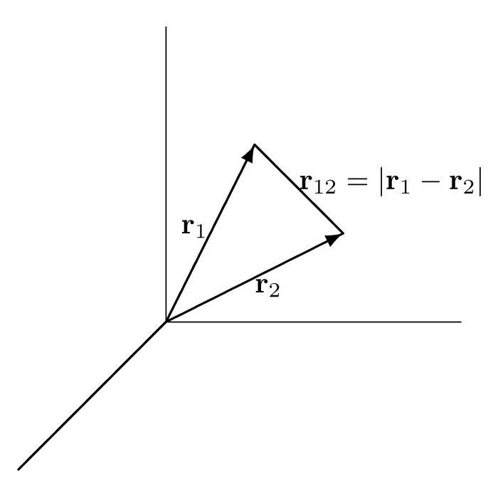
The starting point is the two-electron Schrödinger equation for infinite nuclear mass \begin{equation} \left[-\frac{\hbar^2}{2m}(\nabla^2_1 +\nabla^2_2) - \frac{Ze^2}{r_1} - \frac{Ze^2}{r_2}+\frac{e^2}{r_{12}} \right]\psi = E\psi\nonumber \end{equation} where \(m\) is the electron mass, and \(r_{12} = |{\bf r}_1 - {\bf r}_2|\) (see diagram below).
Begin by rescaling distances and energies so that the Schrödinger equation can be expressed in a dimensionless form. The dimensionless Z-scaled distance is defined by \(\begin{eqnarray} \rho = \frac{Zr}{a_0} \end{eqnarray} \) where \( \begin{eqnarray} a_0 = \frac{\hbar^2}{me^2} \end{eqnarray} \) is the atomic unit (a.u.) of distance equal to the Bohr radius \(0.529\, 177\, 210\, 92(17) \times 10^{-10}\) m. Then
\begin{equation}[-\frac{\hbar^2}{2m}Z^2(\frac{me^2}{\hbar^2})^2(\nabla^2_{\rho_1}+\nabla^2_{\rho_2}) - Z^2\frac{e^2}{a_0}\rho^{-1}_1 - Z^2\frac{e^2}{a_0}\rho^{-1}_2 + \frac{e^2}{a_0}Z\rho^{-1}_{12}]\psi= E\psi\nonumber\end{equation}
But \(\begin{eqnarray} \frac{\hbar^2}{m}(\frac{me^2}{\hbar^2})^2 = \frac{e^2}{a_0} \end{eqnarray} \) is the hartree atomic unit of of energy \((E_h = 27.211\,385\,05(60)\) eV, or equivalently \(E_h/(hc) = 2194.746\,313\,708(11)\) m\(^{-1})\). Therefore, after multiplying through by \(a_0/(Ze)^2\), the problem to be solved in Z-scaled dimensionless units becomes
\begin{equation} [-\frac{1}{2}(\nabla^2_{\rho_1}+\nabla^2_{\rho_2}) - \frac{1}{\rho_1} - \frac{1}{\rho_2} + \frac{Z^{-1}}{\rho_{12}}]\psi = \varepsilon\psi\nonumber \end{equation}
where \(\begin{eqnarray}\varepsilon = \frac{Ea_0}{(Ze)^2} \end{eqnarray}\) is the energy in Z-scaled atomic units. For convenience, rewrite this in the conventional form \begin{equation} H\psi = \varepsilon\psi\nonumber \end{equation} where (using \(r\) in place of \(\rho\) for the Z-scaled distance) \begin{equation} H = -\frac{1}{2}(\nabla^2_1+\nabla^2_2) - \frac{1}{r_1}-\frac{1}{r_2} + \frac{Z^{-1}}{r_{12}} \nonumber\end{equation} is the atomic Hamiltonian for infinite nuclear mass.
The Hartree Fock Method
For purposes of comparison, and to define the correlation energy, assume that \(\psi({\bf r}_1,{\bf r}_2)\) can be written in the separable product form \begin{equation} \psi({\bf r}_1,{\bf r}_2) = \frac{1}{\sqrt{2}} \left[ u_1(r_1) u_2(r_2) \pm u_2(r_1) u_1(r_2) \right] \nonumber \end{equation} for the \(1s^2\ ^1\!S\) ground state. Because of the $\frac{1}{r_{12}}$ term in the Schrödinger equation, the exact solution connot be expressed in this form as a separable product. However, the Hartree-Fock approximation corresponds to finding the best possible solution to the Schrödinger equation \begin{equation} H\psi({\bf r}_1,{\bf r}_2) = E\psi({\bf r}_1,{\bf r}_2)\nonumber \end{equation} that can nevertheless be expressed in this separable product form, where as before \begin{equation} H = -\frac{1}{2}(\nabla^2_1+\nabla^2_2) - \frac{1}{r_1}- \frac{1}{r_2} + \frac{Z^{-1}}{r_{12}}\nonumber \end{equation} is the full two-electron Hamiltonian. To find the best solution, substitute into \(\left\langle\psi \lvert H-E \rvert \psi\right\rangle\) and require this expression to be stationary with respect to arbitrary infinitesimal variations \(\delta u_1\) and \(\delta u_2\) in \(u_1\) and \(u_2\) respectively; i.e.
\begin{equation} \frac{1}{2} \left\langle \delta u_1(r_1)u_2(r_2) \pm u_2(r_1)\delta u_1(r_2) \lvert H-E \rvert u_1(r_1) u_2(r_2)\pm u_2(r_1) u_1(r_2)\right\rangle\nonumber \end{equation}
\begin{equation} =\int\delta u_1(r_1) d{\bf r}_1 \left\{ \int d{\bf r}_2 u_2(r_2) \left( H - E \right) \left[ u_1(r_1)u_2(r_2) \pm u_2(r_1) u_1(r_2) \right] \right\}\nonumber \end{equation}
\begin{equation} = 0 \nonumber \end{equation}
for arbitrary \( \delta u_1(r_1).\nonumber \) Therefore \(\{\int d{\bf r}_2 \ldots \} = 0\).
Similarly, the coefficient of \(\delta u_2\) would give
\begin{equation} \int d{\bf r}_1 u_1(r_1) \left( H-E \right) \left[ u_1(r_1) u_2(r_2) \pm u_2(r_1) u_1(r_2) \right] = 0\nonumber \end{equation}
Define
\begin{equation} I_{12} = I_{21} = \int d{\bf r}\, u_1(r)u_2(r), \nonumber \end{equation}
\begin{equation} H_{ij} = \int d{\bf r}\, u_i(r)(-\frac{1}{2}\nabla - \frac{1}{r})u_j(r), \nonumber \end{equation}
\begin{equation} G_{ij}(r) = \int d{\bf r}^\prime u_i(r^\prime)\frac{1}{|{\bf r} - {\bf r}\prime|}u_j(r^\prime)\nonumber \end{equation}
Then the above equations become the pair of integro-differential equations
\begin{equation} [ H_0 - E + H_{22}+G_{22}(r)]u_1(r) = \mp [ I_{12}(H_0-E) + H_{12}+G_{12}(r)]u_2(r)\nonumber \end{equation}
\begin{equation} [H_0-E+H_{11}+G_{11}(r)]u_2(r) = \mp [I_{12}(H_0-E) + H_{12}+G_{12}(r)]u_1(r)\nonumber \end{equation}
These must be solved self-consistently for the "constants" \(I_{12}\) and \(H_{ij}\) and the function \(G_{ij}(r)\).
The Hartree Fock energy is \(E \simeq -2.87\ldots \)a.u. while the exact energy is \(E = -2.903724\ldots \)a.u.
The difference is called the "correlation energy" because it arises from the way in which the motion of one electron is correlated to the other. The Hartree Fock equations only describe how one electron moves in the average field provided by the other (mean-field theory).
Configuration Interaction
Expand \begin{equation} \psi({\bf r}_1,{\bf r}_2)= C_0u^{(s)}_1(r_1)u^{(s)}_1(r_2) + C_1u^{(P)}_1({\bf r}_1)u^{(P)}_1({\bf r}_2){\cal Y}^0_{1,1,0}(\hat{\bf r}_1, \hat{\bf r}_2)+C_2u^{(d)}_1({\bf r}_1)u^{(d)}_2({\bf r}_2){\cal Y}^0_{2,2,0}(\hat{\bf r}_1, \hat{\bf r}_2)+... \pm \end{equation} exchange where \begin{equation} {\cal Y}^M_{l_1,l_2,L}(\hat{\bf r}_1, \hat{\bf r}_2)=\sum_{m_1,m_2}Y^{m_1}_{l_1}({\bf r}_1)Y^{m_2}_{l_2}({\bf r}_2)\times <l_1l_2m_1m_2\mid LM> \end{equation}
This works, but is slowly convergent, and very laborious. The best CI calculations are accurate to \( ~10^{-7}\) a.u.
Hylleraas Coordinates
[E.A. Hylleraas, Z. Phys. \({\bf 48}, 469(1928)\) and \({\bf 54}, 347(1929)\)] suggested using the co-ordinates \(r_1\), \(r_2\) and \(r_{12}\) or equivalently
\begin{eqnarray} s &=& r_1 + r_2, \nonumber\\ t &=& r_1-r_2, \nonumber\\ u &=& r_{12}\nonumber \end{eqnarray}
and writing the trial functions in the form
\begin{equation} \Psi({\bf r}_1,{\bf r}_2) = \sum^{i+j+k\leq N}_{i,j,k}c_{i,j,k}r_1^{i+l_1}r_2^{j+l_2}r_{12}^ke^{-\alpha r_1 - \beta r_2} \mathcal{Y}^M_{l_1,l_2,L}(\hat{r}_1,\hat{r}_2)\pm \text{exchange}\nonumber \end{equation}
Diagonalizing H in this non-orthogonal basis set is equivalent to solving \( \begin{eqnarray} \frac{\partial E}{\partial c_{i,j,k}} = 0\nonumber \end{eqnarray} \) for fixed \(\alpha\) and \(\beta\).
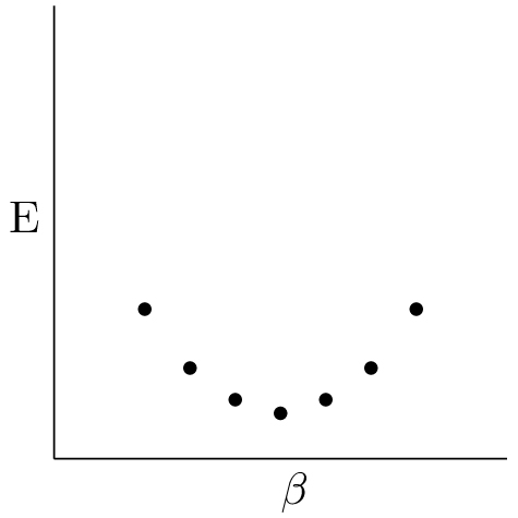
The diagonalization must be repeated for different values of \(\alpha\) and \(\beta\) in order to optimize the non-linear parameters.
Completeness
The completeness of the above basis set can be shown by first writing \(r_{12}^2 = r_1^2 + r_2^2 - 2r_1r_2\cos(\theta_{12})\) and \(\cos(\theta_{12})=\frac{4\pi}{3}\sum^1_{m=-1}Y^{m*}_l(\theta_1,\varphi_1)Y^m_l(\theta_2,\varphi_2)\) consider first S-states. The \(r_{12}^0\) terms are like the ss terms in a CI calculation. The \(r_{12}^2\) terms bring in p-p type contributions, and the higher powers bring in d-d, f-f etc type terms. In general \( P_l(\cos(\theta_{12}) = \frac{4\pi}{2l+1}\sum^l_{m=-l}{Y^{m}_l}^*(\theta_1,\varphi_1)Y^m_l(\theta_2,\varphi_2)\nonumber \)
For P-states, one would have similarly
\(\begin{eqnarray} r_{12}^0\ \ \ \ \ \ \ \ (sp)P\nonumber\\ r_{12}^2\ \ \ \ \ \ \ \ (pd)P\nonumber\\ r_{12}^4\ \ \ \ \ \ \ \ (df)P\nonumber\\ \vdots \ \ \ \ \ \ \ \ \ \ \vdots\nonumber \end{eqnarray}\)
For D-states
\(\begin{eqnarray} r_{12}^0\ \ \ \ \ \ \ \ (sp)D\ \ \ \ \ \ \ \ (pp^\prime)D\nonumber\\ r_{12}^2\ \ \ \ \ \ \ \ (pd)D\ \ \ \ \ \ \ \ (dd^\prime)D\nonumber\\ r_{12}^4\ \ \ \ \ \ \ \ (df)D\ \ \ \ \ \ \ \ (ff^\prime)D\nonumber\\ \vdots \ \ \ \ \ \ \ \ \ \ \vdots\ \ \ \ \ \ \ \ \ \ \ \ \ \ \ \vdots\nonumber\end{eqnarray}\)
In this case, since there are two ``lowest-order couplings to form a D-state, both must be present in the basis set. ie
\(\begin{eqnarray} \Psi(r_2,r_2) = \sum c_{ijk}r_1^ir_2^{j+2}r_{12}^ke^{-\alpha r_1-\beta r-2}\mathcal{Y}^M_{022}(\hat{r}_1,\hat{r}_2)\nonumber\\ +\sum d_{ijk}r_1^{i+1}r_2^{j+1}r_{12}e^{-\alpha^\prime r_1 - \beta^\prime r_2}\mathcal{Y}^M_{112}(\hat{r}_1,\hat{r}_2)\nonumber \end{eqnarray}\)
For F-states, one would need \((sf)F\) and \((pd)F\) terms.
For G-states, one would need \((sg)G\), \((pf)G\) and \((dd^\prime)G\) terms.
Completeness of the radial functions can be proven by considering the Surm-Liouville problem
\( \left(-\frac{1}{2}\nabla^2-\frac{\lambda}{r_s}-E\right)\psi({\bf r}) = 0\nonumber \) or \( \left(-\frac{1}{2}\frac{1}{r^2}\left({r^2}\frac{\partial}{\partial r}\right) - \frac{l\left(l+1\right)}{2r^2} - \frac{\lambda}{r} - E\right)u(r) = 0.\nonumber \) For fixed E and variable \(\lambda\) (nuclear charge).
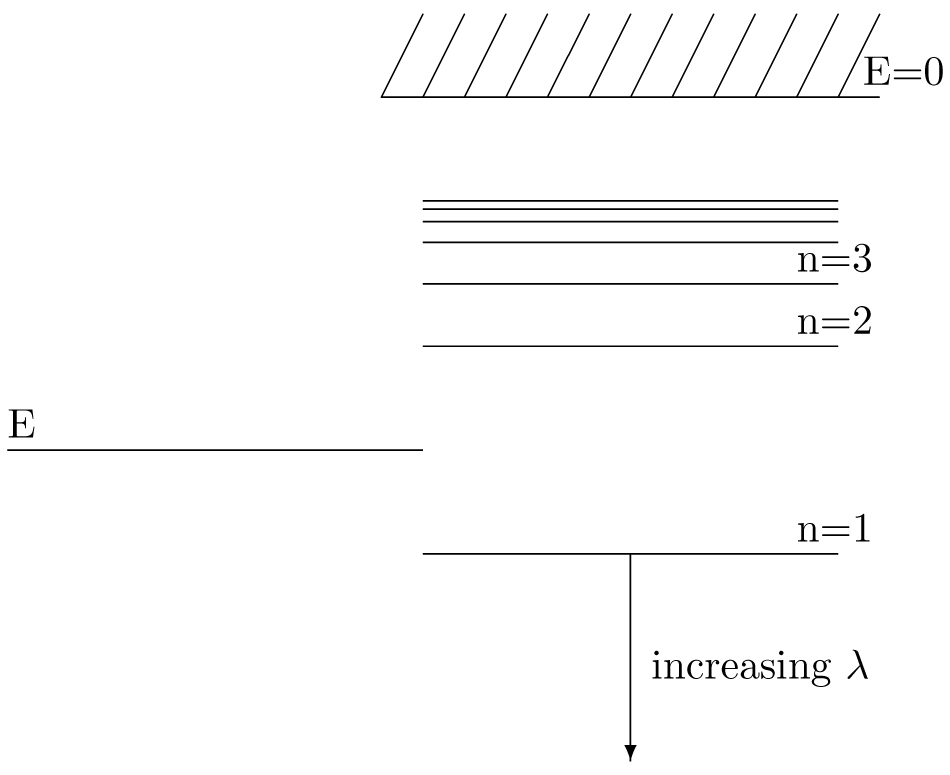
The eigenvalues are \(\lambda_n = (E/E_n)^{1/2}\), where \(E_n =- \frac{1}{2n^2}\)
\( u_{nl}(r) = \frac{1}{(2l+1)!}\left(\frac{(n+l)!}{(n-l-1)2!}\right)^{1/2}(2\alpha)^{3/2}e^{-\alpha r},\nonumber \)
with \(\alpha = (-2E)^{1/2}\) and \(n\geq l+1\).
Unlike the hydrogen spectrum, which has both a discrete part for \(E<0\) and a
continuous part for \(E>0\), this forms an entirely discrete set of finite
polynomials, called Sturmian functions. They are orthogonal with respect to
the potential
-ie \(\int^\infty_0 r^2dru_{n^\prime l}(r)\frac{1}{r}u_{nl}(r) = \delta_{n,n^\prime}\nonumber \)
Since they become complete in the limit \(n\rightarrow\infty\), this assures the
completeness of the variational basis set.
[see B Klahn and W.A. Bingel Theo. Chim. Acta (Berlin) \({\bf 44}, 9\) and \(27 (1977)\)].
Solutions of the Eigenvalue Problem
For convenience, write
\(\Psi({\bf r}_1,{\bf r}_2) = \sum^N_{m=1}c_m\varphi_m\nonumber \)
where \(m= m'th\) combinations of \(i,j,k\)
\(\varphi_{ijk}=r_1^ir_2^jr_{12}^ke^{-\alpha r_1 - \beta r_2}\mathcal{Y}^M_{l_1,l_2,L}(\hat{r}_1,\hat{r}_2) \pm exchange.\nonumber \)
\(
\left( \begin{array}{cc}
\cos(\theta) \sin(\theta)\\
-\sin(\theta) \cos(\theta)
\end{array} \right)
\left( \begin{array}{cc}
H_{11} H_{12}\\
H_{12} H_{22}
\end{array}\right)
\left( \begin{array}{cc}
\cos(\theta) -\sin(\theta)\\
\sin(\theta) \cos(\theta)
\end{array} \right)
= \left(\begin{array}{cc}
cH_{11}+sH_{12} cH_{12} + sH_{22}\\
-sH_{11} + cH_{12} -sH_{12} + cH_{22}
\end{array}\right)
\left( \begin{array}{cc}
c -s\\
s c
\end{array}\right)
= \left(\begin{array}{cc}
c^2H_{11}+s^2H_{22} + 2csH_{12} (c^2-s^2)H_{12}+cs(H_{22}-H_{11})\\
(c^2-s^2)H_{12}+cs(H_{22}-H_{11}) s^2H_{11}+c^2H_{22}-2csH_{12}
\end{array}\right)\)
Therefore \( (\cos^2(\theta)-\sin^2(\theta))H_{12} = \cos(\theta)\sin(\theta)(H_{11}-H_{22})\nonumber \) and \( \tan(2\theta) = \frac{2H_{12}}{H_{11}-H{22}}\nonumber \)
ie
\(\begin{eqnarray} \cos(\theta)=\left(\frac{r+\omega}{2r}\right)^{1/2}\nonumber,\\ \sin(\theta)=-sgn(H_{12})\left(\frac{r-\omega}{2r}\right)^{1/2}\nonumber \end{eqnarray}\\\)
where
\(\begin{eqnarray} \omega = H_{22}-H_{11}\nonumber\\ r=\left(\omega^2+4H_{12}^2\right)^{1/2}\nonumber\\ E_1=\frac{1}{2}\left(H_{11}+H_{22}-r\right)\nonumber\\ E_2=\frac{1}{2}\left(H_{11}+H_{22}+r\right)\nonumber \end{eqnarray}\)
Brute Force Method
-Gives all the eigenvalues and eigenvectors, but it is slow.
-First orthonormalize the basis set - ie form linear combinations
\( \Phi_m = \sum_n\varphi_nR_{nm}\nonumber \) such that \(<\Phi_m|\Phi_n> = \delta_{m,n}\\\). This can be done by finding an orthogonal tranformation, T, such that
\( T^TOT=I=\left( \begin{array}{cccc} \ I_1\ 0 \ldots 0\\ 0\ \ I_2 \ldots 0 \\ \ \ \vdots \ \ \ \ \ \ I_3 \ldots \ 0 \\ 0\ \ 0\ \ 0\ \ddots \end{array}\right); \ \ O_{mn} = <\varphi_m|\varphi_n>\nonumber \) and then applying a scale change matrix \( S = \left(\begin{array}{cccc} \frac{1}{I_1^{1/2}} 0 \ldots 0\\ 0 \frac{1}{I_2^{1/2}} \ldots 0 \\ \vdots \ \ \frac{1}{I_3^{1/2}} 0 \\ 0\ 0\ 0\ \ddots \end{array}\right)= S^T\nonumber \)
Then \(S^TT^TOTS = 1\\\). ie \(R^TOR = 1\) with \(R=TS\).
If H is the matrix with elements \(H_{mn}=<\varphi_m|\varphi_n>\), then H expressed in the \(\Phi_m\) basis set is \( H^\prime = R^THR.\nonumber \)
We next diagonalize \(H^\prime\) by finding an orthogonal transformation W such that \( W^TH^\prime W = \lambda = \left( \begin{array}{cccc} \lambda_1 0 \ldots 0\\ 0\ \lambda_2 \ldots 0 \\ \ \ \vdots \ \ \ \ \ \ddots 0 \\ 0\ \ldots \lambda_N \end{array}\right)\nonumber \)
The q'th eigenvector is
\(\begin{eqnarray} \Psi^{(q)} = \sum_n\Phi_n W_{n,q}\nonumber \\ = \sum_{n,n^\prime}\varphi_{n^\prime}R_{n^\prime ,n}W_{n,q}.\nonumber \end{eqnarray}\) ie. \(c_{n^prime}^{(q)} = \sum_n R_{n^\prime n} W_{n,q}\).
The Power Method
-Based on the observation that if H has one eigenvalue, \(\lambda_M\), much bigger than all the rest, and \(\chi = \left(\nonumber\begin{array}{c}a_1\\a_2\\\vdots\nonumber\end{array}\right)\nonumber\) is an arbitrary starting vector, then \(\chi = \sum_q x_q\Psi^{(q)}\nonumber\).
\(\begin{eqnarray} (H)^n\chi = \sum_q x_q \lambda^n_q\Psi^{(q)}\nonumber\rightarrow x_M\lambda_M^n\Psi^{(M)}\nonumber \end{eqnarray}\\\) provided \(x_M\neq 0\\\).
To pick out the eigenvector correspondng to any eigenvalue, with the original problem in the form
\(\begin{eqnarray} H\Psi = \lambda O\Psi\\\nonumber\\\ (H-\lambda)qO)\Psi\nonumber = (\lambda - \lambda_q)O\Psi\nonumber\end{eqnarray}\)
Therefore, \( G\Psi = \frac{1}{\lambda-\lambda_q}\Psi\nonumber\\ \) where \(G=(H-\lambda_qO)^{-1}O\nonumber\) with eigenvalues \(\frac{1}{\lambda_n-\lambda_q}\nonumber\\\).
By picking \(\lambda_q\) close to any one of the \(\lambda_n\), say \(\lambda_{n^\prime}\), then \(\frac{1}{\lambda_n-\lambda_q}\) is much larger for \(n=n^\prime\nonumber\) than for any other value. The sequence is then
\(\begin{eqnarray} \chi_1=G\chi\nonumber\\ \chi_2=G\chi_1\nonumber\\ \chi_3=G\chi_2\nonumber\\ \vdots\nonumber \end{eqnarray}\\ \)
until the ratios of components in \(\chi_n\) stop changing.
- To avoid matrix inversion and multiplication, note that the sequence is equivalent to
\( F\chi_n = (\lambda-\lambda_q)O\chi_{n-1}\nonumber\\ \)
where \(F = H-\lambda_qO\). The factor of \((\lambda - \lambda_q)\) can be dropped because this only affects the normalization of \(\chi_n\). To find \(\chi_n\\\), solve \( F\chi_n = O\chi_{n-1}\nonumber\\ \) (N equations in N unknowns). Then
\( \lambda = \frac{<\chi_n|H|\chi_n>}{<\chi_n|\chi_n>}\nonumber \)
Matrix Elements of H
\( H=-\frac{1}{2}\nabla^2_1 -\frac{1}{2}\nabla^2_2 - \frac{1}{r_1} - \frac{1}{r_2} +\frac{Z^{-1}}{r_{12}}\nonumber\\ \)
Taking \(r_1, r_2\) and \(r_{12}\) as independent variables,
\(\begin{eqnarray} \nabla_1^2 = \frac{1}{r_1^2}\frac{\partial}{\partial r_1}\left(r_1^2\frac{\partial}{\partial r_1}\right)+ \frac{1}{r_{12}^2}\frac{\partial}{\partial r_{12}} \left(r_{12}^2\frac{\partial}{\partial r_{12}}\right)\nonumber -\frac{l_1(l_1+1)}{r_1^2}+2(r_1-r_2\cos(\theta))\frac{1}{r_{12}}\frac{\partial^2}{\partial r_1 \partial r} \nonumber - 2(\nabla_1 \cdot {\bf r}_2)\frac{1}{r}\frac{\partial}{\partial r}\nonumber \end{eqnarray}\)
where
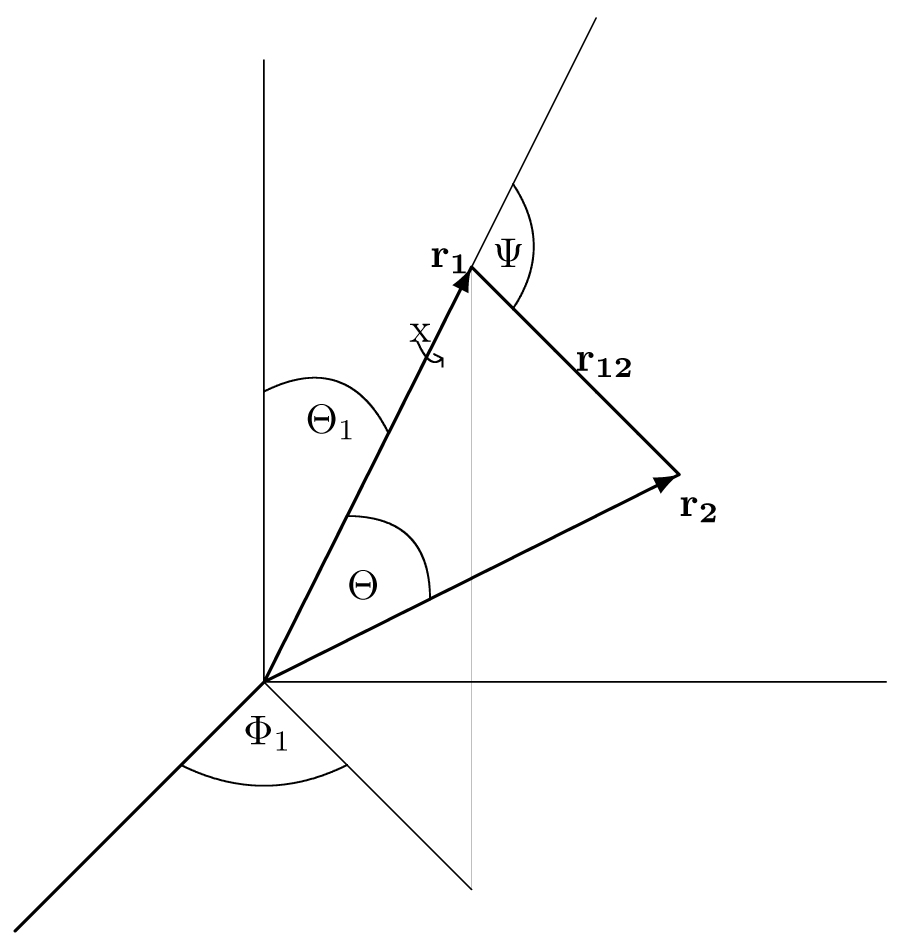
The complete set of 6 independent variables is \(r_1, r_2, r_{12}, \theta_1,\varphi_1, \chi\).
If \(r_{12}\) were not an independent variable, then one could take the column element to be \( d\tau = r_1^2dr_1\sin(\theta_1)d\theta_1d\varphi_1r_2^2dr_2\sin(\theta_2)d\theta_2d\varphi_2.\nonumber \)
However, \(\theta_2\) and \(\varphi_2\) are no longer independent variables. To eliminate them, take the point \({\bf r}_1\) as the
origin of a new polar co-ordinate system, and write \( d\tau=-r_1^2dr_1\sin(\theta_1)d\theta_1d\varphi_1r_{12}^2dr_{12}\sin(\psi)d\psi d\chi\nonumber\\\)
and use \(r_2^2=r_1^2+r_{12}^2 +2r_1r_{12}\cos(\psi).\\ \)
Then for fixed \(r_1\) and \(r_{12}\\\), \( 2r_2dr_2 = -2r_1r_{12}\sin(\psi)d\psi\\ \)
Thus \( d\tau= r_1dr_1r_2dr_2r_{12}dr_{12}\sin(\theta_1)d\theta_1d\varphi_1d\chi\\ \)
The basic type of integral to be calculated is
\(\begin{eqnarray}
I(l_1,m_1,l_2,m_2;R) =\int\sin(\theta_1)d\theta_1d\varphi_1d\chi Y^{m_1}_{l_1}(\theta_1,\varphi_1)^{*}Y^{m_2}_{l_2}(\theta_2,\varphi_2)\nonumber\\
\times\int r_1dr_1r_2dr_2r_{12}dr_{12}R(r_1,r_2,r_{12})\nonumber\\
\end{eqnarray}\\\)
Consider first the angular integral. \(Y^{m_2}_{l_2}(\theta_2,\varphi_2)\\\) can be expressed in terms of the independent variables \(\theta_1, \varphi_1,\chi\\\) by use of the rotation matrix relation
\( Y^{m_2}_{l_2}(\theta_2,\varphi_2) =\sum_m\mathcal{D}^{(l_2)}_{m_2,m}(\varphi_1,\theta_1,\chi)^*Y^m_{l_2}(\theta,\varphi)\nonumber\\\)
where \(\theta, \varphi\) are the polar angles of \({\bf r}_2\) relative to \({\bf r}_1\). The angular integral is then
\(\begin{eqnarray}
I_{ang}=\int^{2\pi}_0d\chi\int^{2\pi}_0d\varphi_1\int^\pi_0\sin(\theta_1)d=theta_1Y^{m_1}_{l_1}(\theta_1,\varphi_1)^*\nonumber\\
\times\sum_m\mathcal{D}^{(l_2)}_{m_2,m}(\varphi_1,\theta_1,\chi)^*Y^m_{l_2}(\theta,\varphi)\nonumber\\
\end{eqnarray}\\\)
Use
\( Y^{m_1}_{l_1}(\theta_1,\varphi_1)^* = \sqrt{\frac{2l_1+1}{4\pi}}\mathcal{D}^{(l_1)}_{m_1,0}(\varphi_1,\theta_1,\chi)\nonumber\\ \)
together with the orthogonality property of the rotation matrices (Brink and
Satchler, p 147)
\( \mathcal{D}^{(j)*}_{m,m^\prime}\mathcal{D}^{(J)}_{M,M^\prime}\sin(\theta_1)d\theta_1d\varphi_1d\chi = \frac{8\pi^2}{2j+1}\delta_{jJ}\delta_{mM}\delta_{m^\prime M^\prime}\nonumber\\ \)
to obtain
\(\begin{eqnarray}
I_{ang}=\sqrt{\frac{2l_1+1}{4\pi}}\frac{8\pi^2}{2l_1+1}\delta_{l_1,l_2}\delta_{m_1,m_2}Y^0_{l_2}(\theta,\varphi)\nonumber\\
=2\pi\delta_{l_1,l_2}\delta_{m_1,m_2}P_{l_2}(\cos\theta)\nonumber\\
\end{eqnarray}\\\)
since
\(Y^0_{l_2}(\theta,\varphi)=\sqrt{\frac{2l_1+1}{4\pi}}P_{l_2}(\cos(\theta))\nonumber\\\).
Note that \(P_{l_2}(\cos\theta)\) is just a short hand expression for a radial function because \(\cos\theta = \frac{r_1^2+r_2^2-r_{12}^2}
{2r_1r_2}\nonumber\\\).
The original integral is thus
\(\begin{eqnarray} I(l_1,m_1,l_2,m_2;R)=2\pi\delta_{l_1l_2}\delta_{m_1m_2}\nonumber\\ \times\int^\infty_0r_1dr_1\int^\infty_0r_2dr_2\int^{r_1+r_2}_{|r_1-r_2|} r_{12}dr_{12}R(r_1,r_2,r_{12})P_{l_2}(\cos\theta)\nonumber\\ \end{eqnarray}\\\)
where \(\cos\theta = (r_1^2 +r^2_2-r_{12}^2)/(2r_1r_2)\nonumber\) is a purely radial function.
The above would become quite complicated for large \(l_2\) because \(P_{l_2}(\cos\theta)\) contains terms up to \((\cos\theta)^{l_2}\\\). However, recursion relations exist which allow any integral containing \(P_l(\cos\theta)\) in terms of those containing just \(P_0(\cos\theta)=1\nonumber\\\)
and \(P_1(\cos\theta)=\cos\theta\nonumber\\\).
Radial Integrals and Recursion Relations
- The basic radial integral is \( I_0(a,b,c) = \int^\infty_0r_1dr_1\int^\infty_{r_1}r_2dr_2\int^{r_1+r_2}_{r_2-r_1}r_{12}dr_{12}r_1^ar_2^br_{12}^ce^{-\alpha r_1-\beta r_2}+\int^\infty_0r_2dr_2\int^\infty_{r_2}r_1dr_1\int^{r_1+r_2}_{r_1-r_2}r_{12}dr_{12}r_1^ar_2^br_{12}^ce^{-\alpha r_1- \beta r_2}\\ =\frac{2}{c+2}\sum^{[(c+1)/2]}_{i=0}\left( c+2 2i+1 \right)\{\frac{q!}{\beta^{q+1}(\alpha+\beta)^{P+1}}\sum_{j=0}q\frac{(p+j)!}{j!}\left(\frac{\beta}{\alpha+\beta}\right)^j+\frac{q^\prime !}{\alpha^{q^\prime+1}(\alpha+\beta)^{p^\prime+1}}\sum^{q^\prime}_{j=0}\frac{(p^\prime+j)!}{j!}\left(\frac{\alpha}{\alpha+\beta}\right)^j\}\nonumber \)
where \( p=a+2i|2\\ p^\prime = b+2i+2\\ q=b+c-2i+2\\ q^\prime = a+c-2i+2 \)
The above applies for a,b \(\geq -2 c\geq -1\). [x] means ``greatest integer in x.
Then \( I_1(a,b,c)=\int d\tau_r r_1^ar_2^br_{12}^ce^{-\alpha r_1-\beta r_2}P_1(\cos\theta) =\frac{1}{2}\left(I_0(a+1,b-1,c)+I_0(a-1,b+1,c)-I_0(a-1,b-1,c+2)\right).\nonumber \)
The Radial Recursion Relation
Recall that the full integral is \(I(l_1m_1,l_2m_2;R)=2\pi\delta_{l_1l_2}\delta_{m_1m_2}I_{l_2}(R)\) where \(I_{l_2}(R) = \int d\tau_r R(r_1,r_2,r_{12})P_{l_2}(\cos\theta)\).
To obtain the recursion relation, use
\(\begin{eqnarray}P_l(x) = \frac{[P^\prime_{l+1}(x)-P^\prime_{l-1}(x)]}{2l+1}\end{eqnarray}\) with \(P_{l+1}^\prime (x) = \frac{d}{dx}P_{l+1}(x)\).
Here \(x=\cos\theta\) and \(\begin{eqnarray}\ \ \ \frac{d}{d\cos\theta}= \frac{dr_{12}}{d\cos\theta}\frac{d}{dr_{12}} = -\frac{r_1r_2}{r_{12}}\frac{d}{dr_{12}}\end{eqnarray}\).
Then, \(\begin{eqnarray}\ \ I_l(R)=-\int d\tau_r R \frac{r_1r_2}{r_{12}}\frac{d}{dr_{12}}\frac{[P_{l+1}(\cos\theta)-P_{l-1}(\cos\theta)]}{2l+1} \end{eqnarray}\).
The \(r_{12}\) part of the integral is \( \begin{eqnarray}\ \ \int^{r_1+r_2}_{|r_1-r_2|}r_{12}dr_{12}R\frac{r_1r_2}{r{12}}\frac{d}{dr_{12}}[P_{l+1}-P_{l-1}]=Rr_1r_2[P_{l+1}-P_{l-1}]^{r_1+r_2}_{|r_1-r_2|}-\int^{r_1+r_2}_{|r_1-r_2|}r_{12}dr_{12}\left(\frac{d}{dr_{12}}R\right)\frac{r_1r_2}{r_{12}}\frac{[P_{l+1}-P_{l-1}]}{2l+1}\nonumber \end{eqnarray}\)
The integrated term vanishes because \(\begin{eqnarray}\ \ \cos\theta = \frac{r_1^2+r_2^2-r_{12}^2}{2r_1r_2}\ \ \ \begin{array}{cc} = -1 & when \ \ r_{12}^2 = (r_1+r_2)^2\\ = \ \ 1 & when \ \ r_{12}^2 = (r_1-r_2)^2 \end{array} \end{eqnarray}\) and \(P_l(1)=1\), \(\ \ P_l(-1)=(-1)^l\).
Thus, \(\begin{eqnarray}\ \ I_{l+1}\left(\frac{r_1r_2}{r_{12}}R^\prime\right) = (2l+1)I_l(R)-I_{l-1}\left(\frac{r_1r_2}{r_{12}}R^\prime\right) \end{eqnarray}\)
If \(R=r_1^{a-1}r_2^{b-1}r_{12}^{c+2}e^{-\alpha r_1 - \beta r_2}\), then \(\begin{eqnarray}\ I_{l+1}(r_1^ar_2^br_{12}^c) = \frac{2l+1}{c+2}I_l(r_1^{a-1}r_2^{b-2}r_{12}^{c+2})+I_{l-1}(r_1^ar_2^br_{12}^c) \end{eqnarray}\)
For the case c=-2, take \(\begin{eqnarray}\ R=r_1^{a-1}r_2^{b-1}\ln r_{12} e^{-\alpha r_1 -\beta r_2}\end{eqnarray}\). Then \(\begin{eqnarray}\ I_{l+1}(r_1^ar_2^br_{12}^c) = I_l(r_1^{a-1}r_2^{b-1}\ln r_{12})(2l+1)-I_{l-1}(r_1^ar_2^br_{12}^{-2}). \end{eqnarray}\) This allows all \(I_l\) integrals to be calculated from tables of \(I_0\) and \(I_1\) integrals.
The General Integral
-The above results fro the angular and raidal integrals can now be combined into a general formula for integrals of the type \(I = \int\int d{\bf r}_1d{\bf r}_2 R_1 \mathcal{Y}^{M^\prime}_{l^\prime_1 l^\prime_2 L^\prime}(\hat{r}_1,\hat{r}_2)T_{k_1k_2K}^Q({\bf r}_1,{\bf r}_2)R_2\mathcal{Y}_{l_ll_2L}^M(\hat{r}_1,\hat{r}_2)\)
where \(\begin{eqnarray} \mathcal{Y}^M_{l_1l_2L}(\hat{r}_1,\hat{r}_2) &=& \sum_{m_1,m_2}<l_1l_2m_1m_2|LM>Y^{m_1}_{l_1}(\hat{r}_1)Y^{m_2}_{l_2}(\hat{r}_2)\nonumber\end{eqnarray}\) and \(\begin{eqnarray} T^Q_{k_1k_2K}({\bf r}_1,{\bf r}_2) &=& \sum_{q_1,q_2}<k_1k_2q_1q_2|KQ>Y_{k_1}^{q_1}(\hat{r}_1)Y^{q_2}_{k_2}(\hat{r}_2)\nonumber \end{eqnarray}\)
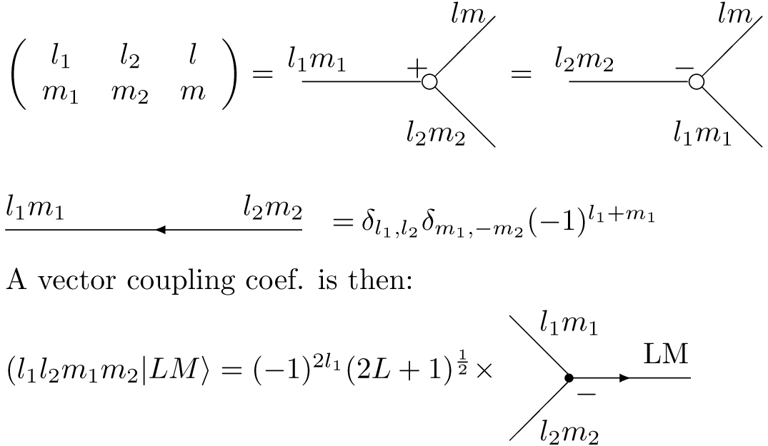
The basic idea is to make repeated use of the formula \(\begin{eqnarray} Y^{m_1}_{l_1}(\hat{r}_1)Y^{m_2}_{l_2}(\hat{r}_2)&=& \sum_{lm}\left(\frac{(2l_1+1)(2l_2+1)(2l+1)}{4\pi}\right)^{1/2}\nonumber\ &\times& \left( \begin{array}{ccc} l_1 & l_2 & l\\ m_1 & m_2 & m\end{array}\right)\left(\begin{array}{ccc} l_1 & l_2 & l\\ 0 & 0 & 0\end{array} \right)Y^{m*}_l(\hat{r}_1)\nonumber \end{eqnarray}\)
where \(Y^{m*}(\hat{r}) = (-1)^mY_l^{-m}(\hat{r})\) and \(\begin{eqnarray} \left(\begin{array}{ccc} l_1 & l_2 & l\\ m_1 & m_2 & m\end{array}\right)= \frac{(-1)^{l_1-l_2-m}}{(2l+1)^{1/2}}(l_1l_2m_1m_2|l,-m) \end{eqnarray}\) is a \(3-j\) symbol.
In particular, write
\(\begin{array}{ccc} Y^{m_2^\prime}_{l_1^\prime}(\hat{r}_1)^*\underbrace{Y_{k_1}^{q_1}(\hat{r}_1)Y^{m_1}_{l_1}(\hat{r}_1)} & = & \sum_{\Lambda M}(\ldots)Y^M_\Lambda(\hat{r}_1)\\ \ \ \ \ \ \ \ \ \ \sum_{\lambda_1\mu_1}Y_{\lambda_1}^{\mu_1}(\hat{r}_1) & &\\ & & \\ Y^{m^\prime}_{l_2^\prime}(\hat{r}_2)\underbrace{Y^{q_2}_{k_2}(\hat{r}_2)Y_{l_2}^{m_2}(\hat{r}_2)} & = & \sum_{\Lambda^\prime M^\prime}(\ldots)Y_{\Lambda^\prime}^{M^\prime *}(\hat{r}_2)\\ \ \ \ \ \ \ \ \ \ \sum_{\lambda_2\mu_2}Y_{\lambda_2}^{\mu_2}(\hat{r}_2) & & \end{array}\)
The angular integral then gives a factor of \(2\pi\delta_{\Lambda,\Lambda^\prime}\delta_{M,M^\prime}P_\Lambda(\cos\theta_{12})\). The total integral therefore reduces to the form \( I = \sum_\lambda C_\Lambda I_\Lambda(R_1R_2), \) where \(c_\Lambda = \sum_{\lambda_1 \lambda_2}C_{\lambda_1,\lambda_2,\Lambda}\).
Graphical Representation
Matrix Elements of H
Recall that \(H = -\frac{1}{2}\nabla^2_1 -\frac{1}{2}\nabla^2_2-\frac{1}{r_1}-\frac{1}{r_2} + \frac{Z^{-1}}{r_{12}}\).
Consider matrix elements of \(\begin{eqnarray} \nabla^2_1 &=& \frac{1}{r_1}^2\left(\frac{\partial}{\partial r_1}\right) + \frac{1}{r^2}\left(\frac{\partial}{\partial r}\right) - \frac{(\vec{l}_1^y)^2}{r_1^2}\nonumber &+&\frac{2(r_1-r_2\cos\theta)}{r}\frac{\partial^2}{\partial r_1 \partial r} - 2(\nabla^y_1\cdot{\bf r}_2)\frac{1}{r}\frac{\partial}{\partial r}.\nonumber \end{eqnarray}\) where \(r \equiv r_{12}\) and \(\cos\theta \equiv \cos\theta_{12}\).
Also \(\hat{\nabla}^y_1 \equiv r_1\nabla^y_1\) operates only on the spherical harmonic part of the wavefunction.
A general matrix element is \(\begin{eqnarray} <r_1^{a^\prime}r_2^{b^\prime}r_{12}^{c^\prime}e^{-\alpha^\prime r_1 -\ beta^\prime r_2}\mathcal{Y}^{M^\prime}_{l^\prime_1l^\prime_2L^\prime}(\hat{r}_1,\hat{r}_2)|\nabla^2_1|r_1^ar_2^br_{12}^ce^{-\alpha r_1 -\beta r_2}\mathcal{Y}^M_{l_1l_2L}(\hat{r}_1,\hat{r}_2)> \end{eqnarray}\).
Since \(\nabla^2_1\) is rotationally invariant, this vanishes unless \(L=L^\prime\), \(M=M^\prime\). Also \(\nabla_1^2\) is Hermitean, so that the result must be the same whether it operates to the right or left, even though the results look very different. In fact, requiring the results to be the same yields some interesting and useful integral identites as follows:
Put \(\begin{eqnarray} \mathcal{F} &=& F \mathcal{Y}^M_{l_1l_2L}(\hat{r}_1,\hat{r_2})\nonumber\end{eqnarray}\), and \(\begin{eqnarray} F &=& r_1^ar_2^br_{12}^ce^{-\alpha r_1 -\beta r_2}.\nonumber \end{eqnarray}\)
Then \(\begin{eqnarray} \nabla^2_1\mathcal{F} &=& [\frac{1}{r_1^2}[a(a+1)-l_1(l_1+1)] + \frac{c(c+1)}{r^2} + \alpha^2\frac{2\alpha(a+1)}{r_1}\nonumber &+& \frac{2(r_1-r_2\cos\theta)}{r_1r^2}c[a-\alpha r_1]-\frac{2c}{r^2}(\hat{\nabla}^y_1\cdot\hat{r}_2)\frac{r_2}{r_1}]\mathcal{F}\nonumber \end{eqnarray}\)
and
\(\begin{eqnarray} <\mathcal{F}^\prime|\nabla^2_1|\mathcal{F}>= \sum_\Lambda \int d\tau_r F^\prime C_\Lambda (1)P_\Lambda(\cos\theta)\{\frac{1}{r_1^2}[a(a+1)-l_1(l_1+1)]\nonumber\\ -\frac{2\alpha(a+1)}{r_1}+\frac{c(c+1)}{r^2} +\alpha^2 + \frac{2(r_2-r_2\cos\theta)}{r_1r^2}c(a-\alpha r_1)\}F\nonumber + \sum_\Lambda\int d\tau_r F^\prime C\Lambda(\hat{\nabla}^y_1\cdot\hat{r}_2)P_\Lambda(\cos\theta)\left(\frac{-2cr_2}{r_1r^2}\right)F\nonumber \end{eqnarray}\)
where \(\begin{eqnarray} \int d\tau_r = \int^\infty_0 r_1 dr_1 \int^infty_0 r_2 dr_2 \int^{r_1+r_2}_{|r_1-r_2|}rdr \end{eqnarray}\).
For brevity, let the sum over \(\Lambda\) and the raidal integrations be
understood, and let \((\nabla_1^2)\) stand for the terms which appear in the
integrand. Then operating to the right gives
\(\begin{eqnarray} (\nabla_1^2)_R &=& \frac{1}{r_1^2}[a(a+1)-l_1(l_1+1)] + \frac{c(c+1)}{r^2} + \alpha^2 - \frac{2\alpha (a+1)}{r_1}\nonumber &+& \frac{2(r_1-r_2\cos\theta)}{r_1r62}c(a-\alpha r_1) - \frac{2cr-2}{r_1r^2}(\hat{\nabla}^y_1\cdot \hat{r}_2)\nonumber \end{eqnarray}\).
Operating to the left gives
\(\begin{eqnarray} (\nabla_1^2)_L &=& \frac{1}{r_1^2}[a^\prime(a^\prime+1)-l_1^\prime(l_1^\prime+1)] + \frac{c^\prime(c^\prime+1)}{r^2} + \alpha^{2^\prime} - \frac{2\alpha^\prime (a^\prime+1)}{r_1}\nonumber &+& \frac{2(r_1-r_2\cos\theta)}{r_1r^2}c^\prime(a^\prime-\alpha r_1) - \frac{2c^\prime r-2}{r_1r^2}({\hat{\nabla}^{y\prime}_1}\cdot \hat{r}_2).\nonumber \end{eqnarray}\)
Now put \( \begin{array}{cccc} a_+ = a+a^\prime, \hat{\nabla}_1^+ = \hat{\nabla}_1^y + \hat{\nabla}_1^{y\prime}\end{array}\) and \(\begin{array}{cccc} a_{-} = a-a^\prime\ \hat{\nabla}_1^{-} = \hat{\nabla}_1^y - \hat{\nabla}_1^{y\prime} \end{array} \) etc.
and substitute \(a^\prime = a_+ - a\), \(c^\prime = c_+ - c\), and \(\alpha^\prime = \alpha_+ - \alpha\) in \((\nabla^2_1)_L\). If \(a_+\), \(c_+\) and \(\alpha_+\) are held fixed, then the equation \( (\nabla^2_1)_R = (\nabla^2_1)_L \) must be true for arbitrary \(a\), \(c\), and \(\alpha\). Their coefficients must thus vanish.
This yields the integral relations \( \label{I} \begin{eqnarray} \frac{(r_1-r_2\cos\theta)}{r_1r^2} = \frac{1}{c_+}\left(\frac{-(a_++1)}{r_1^2}+\frac{\alpha_+}{r_1}\right) \tag{I} \end{eqnarray}\) from the coef. of \(a\), and \( \label{II} \begin{eqnarray} \frac{(r_1-r_2\cos\theta)(a_+-\alpha_+ r_1)}{r_1r^2} = \frac{r_2}{r_1r^2}(\hat{r}_2\cdot\hat{\nabla}_1^+)-\frac{(c_++1)}{r^2} \tag{II} \end{eqnarray}\) from the coef. of \(c\). The coef. of \(\alpha\) gives an equation equivalant to \((I)\).
Furthermore, if can be show that (see problem) \(\begin{eqnarray} \sum_\Lambda \int d\tau_r \frac{r^c}{r^2}C_\Lambda(\hat{r}_2\cdot\hat{\nabla}_1^y)P_\Lambda(\cos\theta) &=&\sum_\Lambda \int d\tau_r \frac{r^c}{cr_1r_2}C\Lambda(1)P_\Lambda(\cos\theta)\nonumber &\times&\left(\frac{l_1^\prime(l_1^\prime+1)-l_1(l_1+1)-\Lambda(\Lambda+1)}{2}\right)\nonumber\end{eqnarray}\)
and similarly for \((\hat{r}_2\cdot\hat{\nabla}^{y\prime}_1)\) with \(l_1\) and \(l_1^\prime\) interchangable, then it follows that \(\begin{eqnarray} \frac{r^{c_+}}{r^2}(\hat{r}_2\cdot\hat{\nabla}_1^+) = -\frac{r^{c_+}}{c_+r_1r_2}\Lambda(\Lambda+1) \end{eqnarray}\)
and \(\begin{eqnarray} \frac{r^{c_+}}{r^2}(\hat{r}_2\cdot\hat{\nabla}_1^-)= \frac{r^{c_+}}{c_+r_1r_2}[l_1^\prime(l_1^\prime+1)-l_1(l_1+1)] \end{eqnarray}\) where equality applies after integration and summation over \(\Lambda\).
Thus \((II)\) becomes \(\begin{eqnarray}\label{IIa} \frac{(r_1-r_2\cos\theta)(a_+-\alpha_+r_1)}{r_1r^2} = -\frac{\Lambda(\Lambda+1)}{c_+r^2_1}-\frac{(c_++1)}{r^2}. \tag{IIa} \end{eqnarray}\)
Problem
Prove the integral relation \(\begin{eqnarray}\ \ \sum_\Lambda \int d\tau_rf(r_1,r_2)\frac{1}{r}\left(\frac{d}{dr}q(r)\right)C_\Lambda(\hat{r}_2\cdot\hat{\nabla}^y_1)P_\Lambda(\cos\theta) =\sum_\Lambda \int d\tau_r \frac{f(r_1,r_2)}{r_1,r_2}q(r)C_\Lambda(1)P_\Lambda(\cos\theta)\nonumber \times \left(\frac{l_1^\prime(l_1^\prime+1)-l_1(l_1+1)-\Lambda(\Lambda+1)}{2}\right).\nonumber \end{eqnarray}\)
where \(C_\Lambda(1)\) are the angular coefficients from the overlap integral \( \int d\Omega \mathcal{Y}^{M*}_{l_1^\prime l_2^\prime L}(\hat{r}_1,\hat{r}_2) = \sum_\Lambda C_\Lambda(1)P_\Lambda(\cos\theta_{12}). \)
Hint: Use the fact that \(l_1^2\) is Hermitean so that \( \int d\tau (l_1^2\mathcal{Y}^\prime)^*q(r)\mathcal{Y} = \int d\tau \mathcal{Y}^{\prime *}l_1^2(q(r)\mathcal{Y}) \) with \(\ \vec{l}_1= \frac{1}{i}\vec{r}_1\times\nabla_1\).
It is also useful to use \(\begin{eqnarray}\ \ (\cos^2\theta-1)P_L(\cos\theta) = \frac{L(L-1)}{(2L-1)(2L+1)}P_{L-2}(\cos\theta)\nonumber =\frac{2(L^2+L-1)}{(2L-1)(2L+3)}P_L(\cos\theta) + \frac{(L+1)(L+2)}{(2L+1)(2L+3)}P_{L+2}(\cos\theta)\nonumber \end{eqnarray}\)
together with the integral recursion relation \( I_{L+1}\left(\frac{1}{r}\frac{d}{dr}q(r)\right) = (2L+1)I_L\left(\frac{1}{r_1r_2}q(r)\right)+I_{L-1}\left(\frac{1}{r}\frac{d}{dr}q(r)\right) \)
Of course \(l_1^2\mathcal{Y}^M_{l_1l_2L}(\hat{r}_1,\hat{r}_2)=l_1(l_1+1)\mathcal{Y}^M_{l_1l_2L}(\hat{r}_1,\hat{r}_2)\).
General Hermitean Property
Each combination of terms of the form \( <f>_R = a^2f_1 af_2+abf_3+b^2f_4+bf_5+af_6\nabla_1^y+bf_7\nabla^y_2+f_8(y) \) can be rewritten \(\begin{eqnarray}\ \ <f>_L= (a_+-a)^2f_1+(a_+-a)f_2 + (a_+-a)(b_+-b)f_3+(b_+-b)^2f_4\nonumber +(b_+-b)f_5+(a_+-a)f_6\nabla^{y\prime}_1+(b_+-b)f_7\nabla^{y\prime}_2+f_8)y^\prime\nonumber \end{eqnarray}\)
Since these must be equal for arbitrary \(a\) and \(b\), \( a_+^2f_1+a_+f_2+_+b_+f_3+b_+f_4+b_+f_5+a_+f_6\nabla^{y\prime}_1 + b_+f_7\nabla^{y\prime}_2+f_8(y^\prime)-f_8(y)=0 \)
Adding the corresponding expresssion with \(y\) and $y^\prime$ interchanged yields \(\label{III} a_+^2f_1+a_+f_2+a_+b_+f_3+b_+^2f_4+b_+f_5+\frac{1}{2}a_+f_6\nabla^+_1+\frac{1}{2}b_+f_7\nabla^+_2=0\tag{III} \)
Subtracting gives \(\label{IV} f_8(y)-f_8(y^\prime)=-\frac{1}{2}[a_+f_6\nabla^-_1+b_+f_7\nabla_2^-]\tag{IV} \) \(\label{V} a[-2a_+f_1-2f_2-b_+f_3-f_6=nabla^+_1]=0\tag{V} \) \(\label{VI} b[-2b_+f_4-2f_5-a_+f_3-f_7\nabla^+_2]=0\tag{VI} \)
Adding the two forms gives
\begin{eqnarray} <f>_R+<f>_L=\frac{1}{2}(a_+^2+a_-^2)f_1+a_+f_2+\frac{1}{2}(a_+b_++a_-b_-)f_3\nonumber\\ \ +\frac{1}{2}(b_+^2+b_-^2)f_4+b_+f_5+\frac{1}{2}f_6(a_+\nabla_1^++a_-\nabla^-_1)\nonumber\\ \ +\frac{1}{2}(b_+\nabla_2^++b_-\nabla^-_2)+f_8(y)+f_8(y^\prime)\nonumber \end{eqnarray}
Subtracting \(\begin{eqnarray}\frac{x}{2}\times(I)\end{eqnarray}\) gives
\begin{eqnarray}\ \ <f>_R+<f>_L = \frac{1}{2}[(1-x)a_+^2 + a_-^2]f_1 + (1-\frac{x}{2})a_+f_2+\frac{1}{2}[(1-x)a_+b_++a_-b_-]f_3\nonumber\\ +\frac{1}{2}[(1-x)b_+^2+b_-^2]f_4+(1-\frac{x}{2})f_5b_++\frac{1}{2}f_6[(1-\frac{x}{2})a_+\nabla_1^++a_-\nabla^-_1]\nonumber\\ +\frac{1}{2}[(1-\frac{x}{2})b_+\nabla^+_2+b_-\nabla^-_2]+f_8(y)+f_8(y^\prime)\nonumber \end{eqnarray}
If \(x=1\), \begin{eqnarray} <f>_R+<f>_L &=& \frac{1}{2}[a_-^2f_1+a_+f_2+a_-b_-f_3+b_-^2f_4+b_+f_5\nonumber\\ &+&\left(\frac{1}{2}a_+\nabla^+_1+a_-\nabla^-_1\right)f_6+\left(\frac{1}{2}b_+\nabla^+_2+b_-\nabla^-_2\right)f_7]+f_8(y)+f_8(y^\prime)\nonumber \end{eqnarray}
The General Hermitean Property for arbitrary \(x\) gives \begin{eqnarray}\ \ \nabla_1^2= \frac{1}{4}\{\frac{1}{r_1^2}[(1-x)a_+^2+a_-^2+2(1-\frac{x}{2})a_+-2[l_1(l_1+1)+l_1^\prime(l_1^\prime+1)]\nonumber\\ -\frac{2}{r_1}[(1-x)\alpha_+a_++\alpha_-a_-+2(1-\frac{x}{2})\alpha_+]+(1-x)\alpha_+^2 + \alpha^2_-]\nonumber\\ +\frac{2(r_1-r_2\cos\theta)}{r_1r^2}[(1-x)(a_+-\alpha_+r_1)c_++(a_--\alpha_-r_2)c_-]\nonumber\\ -\frac{2r_2}{r_1r^2}[(1-\frac{x}{2})c_+\hat{r}_2\cdot\hat{\nabla}_1^++c_-\hat{r}_2\hat{\nabla}_1^-]+\frac{(1-x)c_+^2+c_-^2+2(1-\frac{x}{2})c_+}{r^2}\}\nonumber \end{eqnarray}.
Use \(\begin{eqnarray}\ \ \frac{-2r_2}{r_1r^2}[(1-\frac{x}{2})c_+\hat{r}_2\hat{\nabla}_1^++c_-\hat{r}_2\hat{\nabla}_1^-]=\frac{2}{r_1^2}\left[(1-\frac{x}{2})\Lambda(\Lambda+1)-\frac{c_-}{c_+}[l_1^\prime(l_1^\prime+1)+l_1(l_1+1)]\right]\end{eqnarray}\),
\(\begin{eqnarray} \frac{2(r_1-r_2\cos\theta)}{r_1r^2}(a_--\alpha_-r_1)c_- = 2\frac{c_-}{c_+}\left[\frac{-1}{r_1^2}[a_-(a_++1)]+\frac{1}{r_1}[a_-\alpha_++\alpha_-(a_++2)]-\alpha_-\alpha_+\right]\nonumber \end{eqnarray}\),
and \(\begin{eqnarray}\ \ \frac{2(r_1-r_2\cos\theta)}{r_1r^2}(a_+-\alpha_+r_1)c_+ = 2\left[-\frac{1}{r_1^2}[a_+(a_++1)]+\frac{1}{r_1}[a_+\alpha_++\alpha_+(a_++2)]-\alpha_+^2\right] \end{eqnarray}\).
Substituting into \(\nabla_1^2\) gives
\begin{eqnarray} \nabla^2_1 = \frac{1}{4}\{\frac{1}{r_1^2}[-(1-x)a_+^2 + a_-^2 +xa_+ + 2(1-\frac{x}{2})\Lambda(\Lambda+1)\nonumber\\ -2l_1(l_1+1)(1-\frac{c_-}{c_+}) - 2l_1^\prime(l_1^\prime+1)(1+\frac{c_-}{c_+})-\frac{2c_-a_-}{c_+}(a_++1)]\nonumber\\ - \frac{2}{r_1}\left[-(1-x)\alpha_+(a_++2)+\alpha_-a_-+2(1-\frac{x}{2})\alpha_+ -\frac{c_-}{c_+}[a_-\alpha_++\alpha_-(a_++2)]\right]\nonumber\\ -(1-x)\alpha_+^2+\alpha_-^2-2\frac{c_-}{c_+}\alpha_-\alpha_+ +\frac{1}{r^2}\left[(1-x)c_+^2+c_-^2+2(1-\frac{x}{2})c_+\right]\}\nonumber \end{eqnarray}
This has the form \( \nabla_1^2 = \frac{1}{4}\left[\frac{A_1}{r_1^2}+\frac{B_1}{r_1}+\frac{C_1}{r^2}+D_1\right] \) with
\(\begin{array}{ccc} A_1=-(1-x)a_+^2+a_-^2 +xa_++2(1-\frac{x}{2})\Lambda(\Lambda+1)-2l_1(l_1+1)(1-\frac{c_-}{c_+})\ -2l_1^\prime(l_1^\prime+1)(1+\frac{c_-}{c_+})-\frac{2c_-a_-}{c_+}(a_++1) \ \ \ \ \ \ \ \ \ \ \ \ \ \ \ \ \ \ \ \ \ \ \ \ \ \ \ \ \ \ \ \ \ \ \ \ \ \ \ \ \end{array} \)
\( B_1 = 2\left[(1-x)\alpha_+(a_++2)-\alpha_-a_--2(1-\frac{x}{2})\alpha_++\frac{c_-}{c_+}[a_-\alpha_++\alpha_(a_++2)]\right] \)
\( C_1 = (1-x)c_+^2+ c_-^2 +2(1-\frac{x}{2})c_+ \)
\( D_1 = -1(1-x)\alpha_+^2 +\alpha_-^2 - 2\frac{c_-}{c_+}\alpha_-\alpha_+ \)
The complete Hamiltonian is then (in Z-scaled a.u.)
\(\begin{eqnarray} H =-\frac{1}{2}\nabla^2_1 -\frac{1}{2}\nabla^2_2 -\frac{1}{r_1} -\frac{1}{r_2} +\frac{Z^{-1}}{r}\nonumber\\ = -\frac{1}{2}\nabla^2_1 -\frac{1}{2}\nabla^2_2 -\frac{1}{r_1} -\frac{Z-1}{Zr_2}+Z^{-1}\left(\frac{1}{r}-\frac{1}{r_2}\right)\nonumber\\ \ =-\frac{1}{8}\left[\frac{A_1}{r_1^2}+\frac{B_1+8}{r_1}+\frac{C_1}{r^2}+D_1+D_2 +\frac{A_2}{r_2^2} + \frac{B_2 + 8(Z-1)/Z}{r_2}+\frac{C_2}{r^2}\right]\nonumber + Z^{-1}\left(\frac{1}{r}-\frac{1}{r_2}\right)\nonumber \end{eqnarray}\)
The screened hydrogenic energy is \(\begin{eqnarray} E_{SH}=-\frac{1}{2}\left[\frac{1}{n_1^2}+ \left(\frac{Z-1}{Z}\right)^2\frac{1}{n_2^2}\right] \end{eqnarray}\) so that
\(\begin{eqnarray} H-E_{SH} &=& -\frac{1}{8}[ \frac{A_1}{r_1^2}+\frac{B_1+8}{r_1}+\frac{C_1}{r^2} + D_1 + D_2 -\frac{4}{n_1^2} -\left(\frac{Z-1}{Z}\right)^2\frac{4}{n_2^2}\nonumber +\frac{A_2}{r_2}+\frac{B_2+8(Z-1)/Z}{r_2}+\frac{C_2}{r^2}] + Z^{-1}\left(\frac{1}{r} -\frac{1}{r_2}\right)\nonumber \end{eqnarray}\)
Optimization of Non-linear Parameters
- The traditional method of performing Hylleraas calculations is to write the basis set in the form
\( \Psi = \sum_{i,j,k}c_{i,j,k}\varphi_{i,j,k}(\alpha,\beta)\pm exchange \)
with
\( \varphi_{i,j,k}(\alpha,\beta) = r_1^ir_2^jr_{12}^ke^{-\alpha r_1 - \beta r_2}\mathcal{Y}^M_{l_1l_2L}. \)
The usual procedure is to set \(\alpha = Z\) so that it represents the inner \(1s\) electron, and then to vary \(\beta\) so as to minimize the energy.
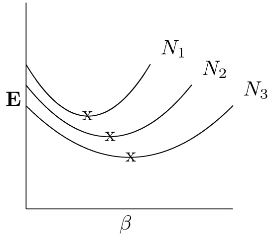
Since \(\beta\) appears in \(\Psi\) as a non-linear parameter, the enitre calculation must be repeated for each value of \(\beta\). However, the minimum becomes progressively smaller as the basis set is enlarged.
- Difficulties
1. If the basis set is constructed so that \( i +j +j \leq N\), the the number of terms is \( (N+1)(N+2)(N+3)/6 \) N=14 already gives 680 terms and an accuracy of about 1 part in \(10^10\) for low-lying states. A substantial improvement in accuracy would require much larger basis sets, together with multiple precision arithmetic to avoid loss of significiant figures when high powers are incluuded.
2. The accuracy rapidly deteriorates as one goes to more highly excited states - about 1 significant figure is lost each time the principle quantum number is increased.
- Cure
We have found that writing basis sets in the form \begin{eqnarray} \Psi &=& \sum_{i,j,k}\left(c^{(1)}_{i,j,k}\varphi_{ijk}(\alpha_1\beta_1) + c_{ijk}^{(2)}\varphi_{ijk}(\alpha_2\beta_2)\right) \pm exchange \nonumber\\ &=& \psi({\bf r}_1,{\bf r}_2) \pm \psi({\bf r}_2,{\bf r}_1)\nonumber \end{eqnarray} so that each combination of powers is includd twice with different non-linear parameters gives a dramatic improvement in accuracy ffor basis sets of about the same total size.
However, the optimization of the non-linear parameters is now much more difficult, and an automated procedure is needed.
If \( E = \frac{<\Psi|H|\Psi>}{<\Psi|\Psi>}, \)
then in \(<\Psi|\Psi> = 1\), \( \frac{\partial E}{\partial\alpha_t} = -2 <\Psi|H-E|r_1\psi({\bf r}_1,{\bf r}_2;\alpha_t)\pm r_21\psi({\bf r}_2,{\bf r}_1;\alpha_t)> \) where \( \psi({\bf r}_1,{\bf r}_2;\alpha_t) = \sum_{i,j,k}c_{ijk}^{(t)}\varphi_{ijk}(\alpha_t\beta_t) \)
- Problem
1. Prove the above.
2. Prove that there is no contribution from the implicit dependence of \(c_{ijk}^{(t)}\) on \(\alpha_t\) if the linear parameters have been optimized.
The Screened Hydrogenic Term
If the Hamiltonian is written in the form (in Z-scaled a.u.) \(\begin{eqnarray}\ H = H_0({\bf r}_1,Z) + H_0({\bf r}_2,Z-1) + Z^{-1}\left(\frac{1}{r}-\frac{1}{r_2}\right) \end{eqnarray}\) with \(\ H_0({\bf r}_1,Z) = -\frac{1}{2}\nabla_1^2 - \frac{1}{r_1}\nonumber \) and \( H_0({\bf r}_2,Z-1) = -\frac{1}{2}\nabla_2^2 - \frac{Z-1}Z{r_2}\nonumber \), then the eigenvectors of \(H_0({\bf r},Z) +H_0({\bf r}_2,Z-1)\) are products of hydrogenic orbitals \( \Psi_0=\psi_0(1s,Z)\psi_0(nl,Z-1) \) and the eigenvalue is \(\begin{eqnarray} E_{SH} = \left[-\frac{1}{2} - \left(\frac{Z-1}{Z}\right)^2\frac{1}{2n^2}\right]Z^2 a.u. \end{eqnarray}\) called the screened hydrogenic eigenvalue. From highly excited states, \(E_{SH}\) and \(\Psi_0\)are already excellent approximations.
For example, for the 1s8d states, the energies are
\(\begin{eqnarray}\\ E(1s8d^1D)= -2.00781651256381 a.u.\nonumber\\ E(1s8d^3D)= - 2.00781793471171 a.u.\nonumber\\ E_{SH} = -2.0078125\nonumber \end{eqnarray}\)
It is therefore advantageousto include the screened hydrogenic terms in the basis set so that the complete trial function becomes \( \Psi = c_0\Psi_0 + \sum_{ijk}\left[c_{ijk}^{(1)}\varphi_{ijk}(\alpha_1,\beta_1)+c_{ijk}^{(2)}\varphi(\alpha_2,\beta_2)\right]\pm exchange \)
Also, the variational principal can be re-expressed in the form \(\begin{eqnarray} E= E_{SH}+\frac{<\Psi|H-E_{SH}|\Psi>}{<\Psi|\Psi>} \end{eqnarray}\) so that the \(E_{SH}\) term can be cancelled analytically from the matrix elements.
For example \( <\Psi_0|H-E_{SH}|\Psi_0> = 0 \)
and \( <\varphi_{ijk}|H-E_{SH}|\Psi_0> = Z^{-1}<\varphi_{ijk}|\frac{1}{r}-\frac{1}{r_2}|\Psi_0> \)
Recall that \(\begin{eqnarray}\ \ I_0(a,b,c) = \frac{2}{c+2}\sum^{[c+1]/2}_{i=0}\left(\begin{array}{c} c+2\\ 2i+1 \end{array}\right) \left[f(p,q;\beta) + f(p^\prime,q^\prime;\alpha)\right] \end{eqnarray}\) where
\(\begin{eqnarray} f(p,q;x) = \frac{q!}{x^{q+1}(\alpha+\beta)^{p+1}}\sum^p_{j=0}\frac{(p+j)!}{j!}\left(\frac{x}{\alpha+\beta}\right)^j \end{eqnarray}\)
\( \begin{array}{cc} p=a+2i+2 & p^\prime = b+2i+2\\ q= b+c-2i+2 & q^\prime =a+c-2i+2 \end{array} \)
If \(\beta\ll\alpha\), the \(f(p,q;\beta)\gg f(p^\prime,q^\prime;\alpha)\) and the \(i=0\) term is the dominant contribution to \(f(p,q;\beta)\). However, since this term depends only on the sum of powers \(b+c\) for \(r_2\), it cancels exactly from the matrix element of \(\begin{eqnarray}\frac{1}{r_12} - \frac{1}{r_2}\end{eqnarray}\) and can therefore be omitted in the calculations of integrands, there by saving many significant figures. This is especially valuable when \(b+c\) is large and \(a\) is small.
Small Corrections
- Mass Polarization
If the nuclear mass is not taken to be infinite, then the Hamiltonian is \(\begin{eqnarray}\ \ H = \frac{P_N^2}{2M} + \sum_{i=1}\frac{p_i^2}{2m} + V \end{eqnarray}\)
where \(M =M_A-nm\) is the nuclear mass and \(m\) is the electron mass.
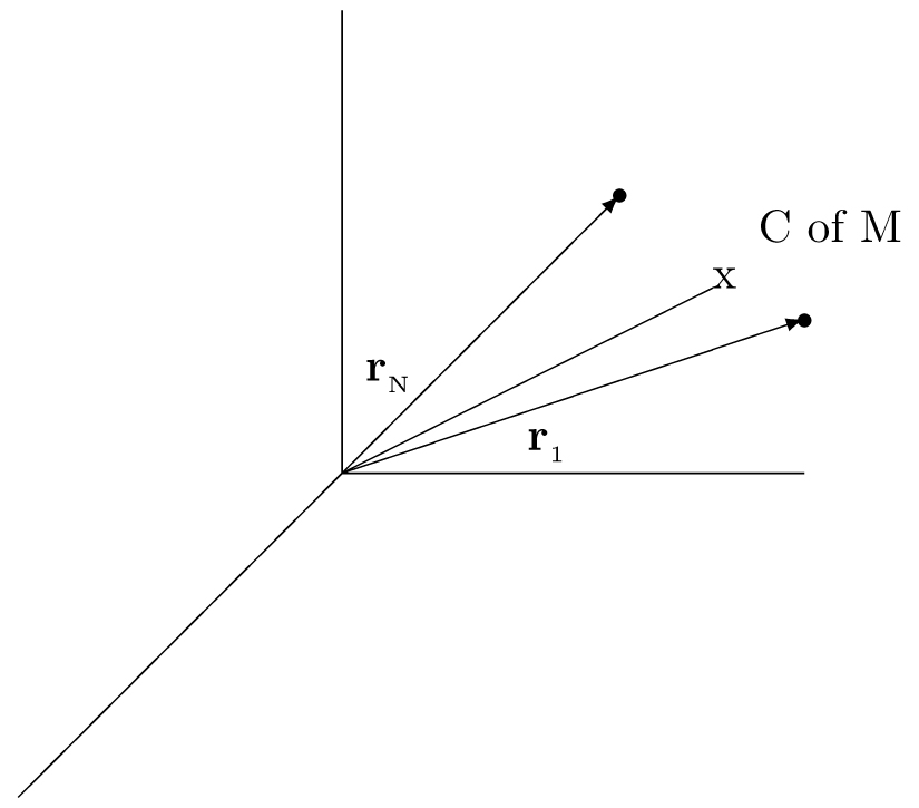
Change variables to the C of M \(\begin{eqnarray} {\bf R} = \frac{1}{M+nm}\left[M{\bf r}_N + m({\bf r}_1 + {\bf r}_2 + \ldots)\right] \end{eqnarray}\)
and relative variables
\( {\bf s}_i = {\bf r}_i - {\bf r}_N. \)
Then
\(\begin{eqnarray}\ \ \ \ \ H = \frac{1}{2(M+nm)}{\bf p}_R^2+\frac{1}{2m}\sum_{i=1}^n{\bf p}_{s_i}^2 +\frac{1}{2M}\sum_{i,k}{\bf p}_{s_i}\cdot {\bf p}_{s_k} + V({\bf s}_1, {\bf s}_2, \ldots)\nonumber = \frac{1}{M+nm}{\bf p}_R^2+\frac{1}{2\mu}\sum_{i=1}^n{\bf p}_{s_i}^2+\frac{1}{2M}\sum_{i\neq k}{\bf p}_{s_i}\cdot {\bf p}_{s_k}+V({\bf s}_1, {\bf s}_2, \ldots)\nonumber \end{eqnarray}\)
where \(\begin{eqnarray} \mu = \left(\frac{1}{M} + \frac{1}{m}\right)^{-1} \end{eqnarray}\)
If \(n=2\), the Schroedinger equation is \(\begin{eqnarray}\ \ \ \left[ -\frac{\hbar^2}{2\mu}(\nabla^2_{s_1}+ \nabla^2_{s_2}) - \frac{\hbar^2}{M}\nabla_{s_1}\nabla_{s_2}-\frac{Ze^2}{s_1}-\frac{Ze^2}{s_2}+\frac{e^2}{s_12}\right]\psi = E\psi \end{eqnarray}\).
Define the reduced mass Bohr radius \(\begin{eqnarray} a_\mu = \frac{hbar^2}{\mu e^2} = \frac{m}{\mu}a_0 \end{eqnarray}\) and
\(\begin{eqnarray} \rho_i = \frac{Zs_i}{a_\mu}\nonumber\\ \varepsilon = \frac{E}{Z^2(e^2/a_\mu)}\nonumber \end{eqnarray}\)
The Schroedinger equation then becomes \(\begin{eqnarray}\ \ \ \left[ -\frac{1}{2}(\nabla^2_{\rho_1}+\nabla^2_{\rho_2})-\frac{\mu}{M}\vec{\nabla}_{\rho_1}\cdot\vec{\nabla}_{\rho_2} - \frac{1}{\rho_1}-\frac{1}{\rho_2}+\frac{Z^{-1}}{\rho_{12}}\right]\psi = \varepsilon \psi \end{eqnarray}\)
The effects of finite meass are thus
1. A reduced mass correction to all energy levels of \((e^2/a\mu)/(e^2/a_0) = \mu/m\), ie. \(\begin{eqnarray} E_M=\frac{\mu}{m}E_\infty \end{eqnarray}\)
2. A specific mass shift given in first order perturbation theory by \(\begin{eqnarray} \Delta\varepsilon = -\frac{\mu}{M}<\psi|\nabla_{\rho_1}\cdot\nabla_{\rho_2}|\psi> \end{eqnarray}\) or
\(\begin{eqnarray} \Delta\varepsilon = -\frac{\mu}{M}<\psi|\nabla_{\rho_1}\cdot\nabla_{\rho_2}|\psi>\frac{e^2}{a_\mu}\nonumber\\ = -\frac{\mu^2}{mM}<\psi|\nabla_{\rho_1}\cdot\nabla_{\rho_2}|\psi>\frac{e^2}{a_0}\nonumber \end{eqnarray}\)
Since \(\nabla_{\rho_1}\cdot\nabla_{\rho_2}\) has the same angular properties as \({\bf\rho}_1 \cdot {\bf\rho}_2\), the operator is like the product of two dipole operators. For product type wave functions of the form \( \psi = \psi(1s)\psi(nl) \pm exchange \) the matrix element vanishes for all but p-states.
